A Basic Introduction

In the following introduction, we showcase some common use cases of PineAPPL that are available through the Python interface. For more details about all the available functionalities, refer to the API documentation.

Setting up

In order to start using PineAPPL, one first needs to install it. The easiest way to install the latest stable version is via pip using the following command:

pip install pineappl

In order to check that PineAPPL was installed properly, one can try to import it:

[1]:

import pineappl

If the above command was successful (did not result in an error), we can download the PineAPPL grid that will be used throughout this tutorial.

[2]:

!wget --no-verbose --no-clobber 'https://data.nnpdf.science/pineappl/test-data/LHCB_DY_8TEV.pineappl.lz4'

We can now load the downloaded grid by running the following:

[3]:

# Load the PineAPPL grid
grid = pineappl.grid.Grid.read("./LHCB_DY_8TEV.pineappl.lz4")

NOTE: For the pineappl.grid.Grid.read() function, both .pineappl and .pineappl.lz4 extensions are acceptable, as long as they are consistent. Without the .lz4 extension, the grid is assumed to not be compressed.

How can I convolve a given PineAPPL grid with a PDF?

[4]:

# We first need to load the PDF set with LHAPDF
import lhapdf
import numpy as np

# `Polars` is a better alternative to Pandas (written in Rust!)
# If you don't have it installed. Simply run `pip install polars`
import polars as pl

lhapdf.setVerbosity(0)
# Choose the PDF set to be used
pdfset = "NNPDF40_nnlo_as_01180"
# Use the central PDF, ie. member ID=0
pdf = lhapdf.mkPDF(pdfset, 0)

In order to convolve a grid, we need to specify the types of convolutions that are required. This includes the polarization and the PDG IDs of the involved hadrons, as well as wether or not the hadron is in the initial- or final-state.

In our example, the grid involves two initial-state unpolarized protons. We can therefore construct the convolution types as follows:

[5]:

from pineappl.convolutions import Conv, ConvType

conv_type = ConvType(polarized=False, time_like=False)
conv_object = Conv(convolution_types=conv_type, pid=2212)

Our grid can now be convolved with our PDF set using the convolve() function.

[6]:

predictions = grid.convolve(
    pdg_convs=[conv_object, conv_object],  # Similar convolutions for symmetric protons
    xfxs=[pdf.xfxQ2, pdf.xfxQ2],  # Similar PDF sets for symmetric protons
    alphas=pdf.alphasQ2,
)
df_preds = pl.DataFrame(
    {
        "bins": range(predictions.size),
        "predictions": predictions,
    }
)
df_preds

[6]:

shape: (18, 2)

bins	predictions
i64	f64
0	8.159231
1	23.890855
2	38.306994
3	51.278627
4	62.349204
…	…
13	22.640245
14	12.927123
15	6.138797
16	1.435175
17	0.052598

We can see that convolve() can perform convolutions with an arbitrary number of distributions. This is why pdf_convs and xfxs are lists that respectively take all the types of convolutions and distributions corresponding to the involved hadrons.

NOTE: If the hadrons have the same type of convolutions and require the convolution to the same distribution, then only one single element can be passed to the list:

# Pass the shared convolution type and distribution to all hadrons
predictions = grid.convolve(
    pdg_convs=[conv_object],
    xfxs=[pdf.xfxQ2],
    alphas=pdf.alphasQ2,
)

The length of predictions is the same as the number of bins that define the observable in question. In our example, it is the inclusive cross-section for Z boson production in bins of the muon pseudorapidity at 8 TeV. See arXiv:1511.08039 for more details, with the corresponding HepData tables.

To see that our predictions are consistent with the experimental measurements, we can plot a comparison of the two using only the central values.

[7]:

import matplotlib.pyplot as plt

# Experimental central values as provided by HepData
data_central = np.array(
    [
        1223.0,
        3263.0,
        4983.0,
        6719.0,
        8051.0,
        8967.0,
        9561.0,
        9822.0,
        9721.0,
        9030.0,
        7748.0,
        6059.0,
        4385.0,
        2724.0,
        1584.0,
        749.0,
        383.0,
        11.0,
    ]
)

# Normalization for each bin. See Section below for more details.
bin_norm = np.array([0.125 for _ in range(predictions.size - 2)] + [0.250, 0.250])

fig, ax = plt.subplots(figsize=(5.6, 3.9))
# Factor of `1e3` takes into account the unit conversion into `fb`
ax.plot(
    df_preds["bins"],
    1e3 * bin_norm * df_preds["predictions"],
    "s",
    markersize=8,
    label="theory",
)
ax.plot(df_preds["bins"], data_central, "o", markersize=8, label="data")
ax.grid(True, alpha=0.5)
ax.set_yscale("log")
ax.set_xlabel("bins")
ax.set_ylabel(r"$d\sigma / dy_\mu$ (fb)")
ax.legend()

plt.show()

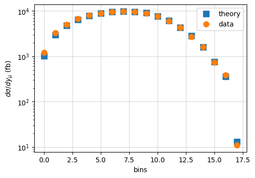
As we can see, the theory predictions agree fairly well with the experimental measurements. However, in order to have a meaningful comparison, one needs to include all sources of experimental and theory uncertainties. Notice that in the plot above, we are accounting for the change in normalization related to each bin, something that we can directly modify inside the PineAPPL grid as we will see later.

NOTE: As mentioned before, if the two initial state hadrons are different (as is the case in \(pp\) collisions in which one of the protons is polarized), then one can convolve the grid with two different PDF sets using the convolve() function:

# Define the convolution types for each of the (un)polarized hadrons
pol_type = ConvType(polarized=True, time_like=False) # `polarized = True`
pol_object = Conv(convolution_types=pol_type, pid=2212)

unpol_type = ConvType(polarized=False, time_like=False)
unpol_object = Conv(convolution_types=conv_type, pid=2212)

# Convolve the two initial state hadrons with different PDF sets
predictions = predictions = grid.convolve(
    pdg_convs=[pol_object, conv_object],
    xfxs=[polarized_pdf.xfxQ2, 2212, unpolarized_pdf.xfxQ2],
    alphas=pdf.alphasQ2,
)

NOTE: The same function convolve also works for convolving FK tables with PDF sets.

How can I get information on the contents of a given PineAPPL grid?

Once the PineAPPL grid is loaded, one can look into its contents and modify them. Below we illustrate how to extract the most common information from a given grid.

Contributing channels

[8]:

# To get all the contributing channels
for idx, c in enumerate(grid.channels()):
    print(f"{idx}: {c}")

0: [([2, -2], 1.0), ([4, -4], 1.0)]
1: [([0, -4], 1.0), ([0, -2], 1.0)]
2: [([22, -4], 1.0), ([22, -2], 1.0)]
3: [([2, 0], 1.0), ([4, 0], 1.0)]
4: [([2, 22], 1.0), ([4, 22], 1.0)]
5: [([1, -1], 1.0), ([3, -3], 1.0)]
6: [([0, -3], 1.0), ([0, -1], 1.0)]
7: [([22, -3], 1.0), ([22, -1], 1.0)]
8: [([1, 0], 1.0), ([3, 0], 1.0)]
9: [([1, 22], 1.0), ([3, 22], 1.0)]
10: [([5, -5], 1.0)]
11: [([0, -5], 1.0)]
12: [([22, -5], 1.0)]
13: [([5, 0], 1.0)]
14: [([5, 22], 1.0)]
15: [([22, 22], 1.0)]
16: [([-5, 22], 1.0), ([-3, 22], 1.0), ([-1, 22], 1.0)]
17: [([1, 22], 1.0), ([3, 22], 1.0), ([5, 22], 1.0)]

The above prints out all the contributing channels where the first two elements of the tuple represent the particle PID (following the PDG conventions). For instance, in the first entry, the up-antiup (2,-2) and charm-anticharm (4,-4) initial states are merged together, each with a multiplicative factor of 1. In general this number can be different from 1, if the Monte Carlo decides to factor out CKM values or electric charges.

Perturbative orders

[9]:

# To get the information on the orders:
orders = []
for idx, o in enumerate(grid.orders()):
    orders.append(o.as_tuple())

df_orders = pl.DataFrame(np.array(orders), schema=["as", "a", "lf", "lr", "la"])
df_orders.with_row_index("Index")

[9]:

shape: (7, 6)

Index	as	a	lf	lr	la
u32	i64	i64	i64	i64	i64
0	0	2	0	0	0
1	1	2	0	0	0
2	1	2	1	0	0
3	1	2	0	1	0
4	0	3	0	0	0
5	0	3	1	0	0
6	0	3	0	1	0

The table above lists the perturbative orders contained in the grid where the powers of the strong coupling \(a_s\), the electroweak coupling \(a\), the factorization \(\ell_F = \log(\mu_F^2/Q^2)\), renormalization \(\ell_R=\log(\mu_R^2/Q^2)\), and fragmentation \(\ell_A=\log(\mu_A^2/Q^2)\) logs are shown. For instance, the first index shows that the grid contains a leading-order (LO) which has the coupling \(a_s^2\).

Observable binning

Grids often correspond to an dataset, which correspond to an observable measured at several kinematic configurations, or bins. The bins might be just 1 dimensional, as is the case here with rapidity, or for more complicated measurements higher dimensional. Each bin is characterized by its left and right border.

[10]:

# To get the bin configurations
bin_dims = grid.bin_dimensions()

# Get the bin specifications.
bin_specs = np.array(grid.bin_limits())

# Each element of bins is an object with a left and right limit and
# an associated bin normalization.
df = pl.DataFrame({})
for bin_dim in range(bin_dims):
    df = pl.concat(
        [
            df,
            pl.DataFrame(
                {
                    f"dim {bin_dim} left": bin_specs[:, bin_dim, 0],
                    f"dim {bin_dim} right": bin_specs[:, bin_dim, 1],
                }
            ),
        ],
        how="vertical",
    )
df

[10]:

shape: (18, 2)

dim 0 left	dim 0 right
f64	f64
2.0	2.125
2.125	2.25
2.25	2.375
2.375	2.5
2.5	2.625
…	…
3.625	3.75
3.75	3.875
3.875	4.0
4.0	4.25
4.25	4.5

How can I edit a grid?

Sometimes it is required to modify the contents of a grid for various reasons (like plotting for example, as we saw earlier). The contents of PineAPPL grids can be edited in various ways. In our example, we are going to change the normalization related to each bin in order for our observable to match the experimental measurements (see Section above).

Let us first check the normalizations before we modify them:

[11]:

df_bins = pl.DataFrame({"bin normalization": grid.bin_normalizations()})
df_bins.with_row_index()

[11]:

shape: (18, 2)

index	bin normalization
u32	f64
0	0.125
1	0.125
2	0.125
3	0.125
4	0.125
…	…
13	0.125
14	0.125
15	0.125
16	0.25
17	0.25

The column bin normalization shows the factor that all convolutions are divided with. In our case, these values should be 1 in order to match the experimental measurements.

[12]:

# Import the Module to set bin specifications
from pineappl.boc import BinsWithFillLimits

# Extract the left & right bin limits
bin_limits = [
    [(bin_specs[b, d, 0], bin_specs[b, d, 1]) for d in range(bin_dims)]
    for b in range(grid.len())
]

# Set the normalization factor to `1`
normalizations = [1.0 for _ in grid.bin_normalizations()]

# Instantiate the bin spec object
bin_configs = BinsWithFillLimits.from_limits_and_normalizations(
    limits=bin_limits,
    normalizations=normalizations,
)

# Set the updated bin configurations
grid.set_bwfl(bin_configs)

# Save the modified grid
grid.write_lz4("./LHCB_DY_8TEV_custom_normalizations.pineappl.lz4")

We can now check that the normalizations have indeed been changed:

[13]:

# Load our modified grids
grid_nrm = pineappl.grid.Grid.read("./LHCB_DY_8TEV_custom_normalizations.pineappl.lz4")
df_nbins = pl.DataFrame({"bin normalization": grid_nrm.bin_normalizations()})
df_nbins.with_row_index()

[13]:

shape: (18, 2)

index	bin normalization
u32	f64
0	1.0
1	1.0
2	1.0
3	1.0
4	1.0
…	…
13	1.0
14	1.0
15	1.0
16	1.0
17	1.0

Fast-Kernel (FK) tables

Fast-kernel (FK) tables are a special kind of grid, which contain the Evolution Kernel Operators (EKO) which encode the DGLAP evolution equations. Furthermore, FK tables do not have perturbative orders while PineAPPL grids do.

You can load them as well, using the FK interface:

# Loading a FK table
fk = pineappl.fk_table.FkTable.read("path/to/fktable.pineappl.lz4")